













Optical Computing in Financial Applications
Optical Computing in Financial Applications
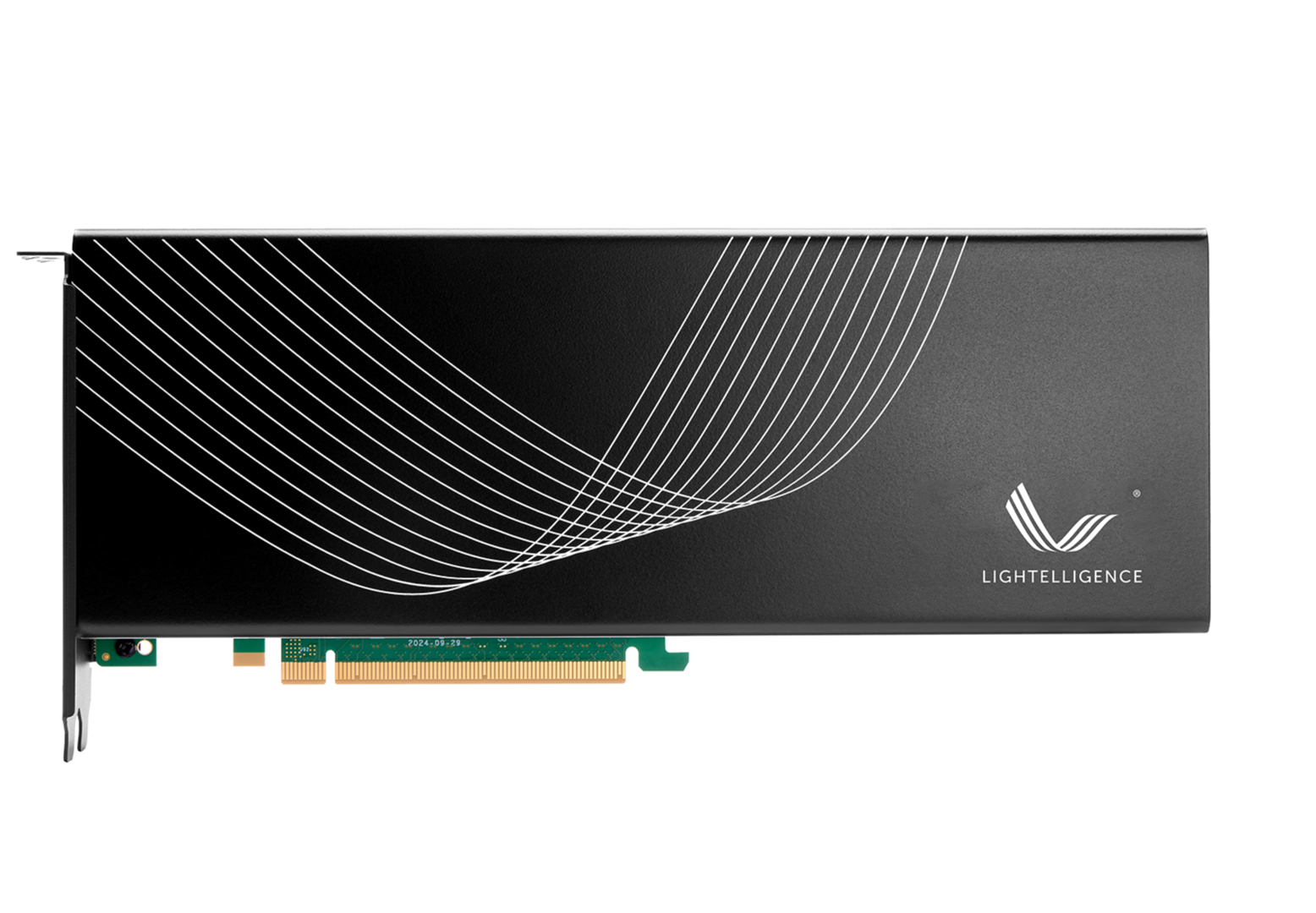
Lightelligence’s Optical Computing Chip
Lightelligence’s optical computing chip incorporates an array of optical matrix multipliers. By leveraging the principle of fast light propagation in photonic devices, it achieves the advantages of high throughput, low latency, and low power consumption. It can be applied to rapidly solve NP-complete problems, such as the maximum clique problem.
In 2021, Lightelligence introduced the PACE (Photonic Arthetric Computing Engine) optical computing processor. At its core is a 64×64 optical matrix multiplier, built by stacking an integrated silicon photonic chip and a CMOS microelectronic chip in a 3D package. A single photonic chip integrates over 10,000 photonic devices. Operating at a 1 GHz system clock, it can solve Ising problems, max-cut/min-cut problems, and maximum clique problems up to hundreds of times faster than today’s high-end GPUs. Detailed parameters are shown in Table 1 below.
| Table 1: PACE Parameter Values | |
| Parameter content | Numerical value |
Computing core | 64x64光Optical matrix multiplier |
| Numerical precision | 7bit(Effective calculation accuracy) |
| Theoretical peak computing power | 8Tops |
| Consumption | 2W |
| Energy efficiency ratio | 4Tops/W |
| (oMAC)Latency | 150ps |
Accelerating Matrix Multiplication with Optical Computing
Matrix multiplication is a typical linear operation that can be accelerated using photonic linear computing units. Programmable optical matrix computation (Optical Multiply-Accumulate, oMAC) is expected to sustain continued growth in computing power even after Moore’s Law reaches its limits, providing robust hardware infrastructure for the digital economy era.
oMAC (Optical Multiply-Accumulate)
For each optical multiply-accumulate operation, the input vector values are first fetched from on-chip memory, converted to analog values by digital-to-analog converters, and applied to the corresponding optical modulators through microbumps between the electronic chip and the photonic chip, forming an input optical vector. This input optical vector then propagates through an optical matrix, producing an output optical vector, which reaches an array of photodetectors that convert the light intensity into electrical current signals. Finally, the electrical signals return to the electronic chip through the microbumps, passing through transimpedance amplifiers and analog-to-digital converters to return to the digital domain.
Low Latency
Compared to traditional CMOS digital circuits, the most significant advantage of optical matrix computing is low latency. Since the computation process is essentially the propagation of optical signal arrays through the chip, the computation latency can be regarded as the time it takes for light to travel through the chip, typically under 1 ns. As shown in Figure 3, for an N×N systolic matrix computing unit, the latency is proportional to O(N). Some latency-optimized architectures can achieve latency close to O(logN) when the matrix size is small. In contrast, the time consumed by optical matrix computing mainly comes from optical-to-electrical conversion and digital-to-analog conversion, which generally takes several clock cycles and is nearly independent of matrix size—equivalent to O(1). A single optical matrix computation can achieve latency below 3 ns. Therefore, for large N, the latency advantage of optical matrix computing is very pronounced. Moreover, traditional digital computing using relatively mature processes such as 28 nm struggles to achieve a global clock frequency above 1 GHz, whereas the control circuitry for optical matrix computing can reach frequencies of several GHz with relative ease, further enhancing the latency advantage.
Low Power Consumption
In addition to the latency advantage, optical computing also features low energy consumption. For an N×N digital matrix computing unit, energy consumption is k×N, where k relates to the power of a single multiply-accumulate operation, proportional to O(N). For an optical matrix multiplier, its power consumption can be expressed as k₁×N + k₂×N², where k₁ is associated with the power of the vector input and receiving ends, and k₂ is associated with the power of the matrix weight section. When the matrix refresh rate is much lower than the signal input rate, the energy consumption is dominated by the first part, making it proportional to O(N). With well-optimized optical devices and their control circuits, the energy efficiency of optical computing based on relatively traditional process nodes can match or even surpass that of digital chips built on advanced process nodes.
Case Study: Option Pricing for Financial Derivatives
The “Snowball” structure is a path-dependent exotic derivative with a relatively complex structure. Since 2019, this non-principal-protected Snowball structured note has drawn increasing attention in the market, with various financial institutions participating in different roles, and its influence has gradually expanded. A Snowball structured note is essentially a put option with a knock-in structure that has been sold. As long as the underlying asset does not experience a significant decline, the longer the note is held, the more coupon income it accrues—much like a snowball rolling downhill, as long as there are no large pits in the ground, it keeps growing bigger.
It is easy to see why Snowball products are so popular: this popularity is largely due to their fixed-income-like characteristics. In a market environment of generally declining interest rates, very few products can offer an annualized coupon of around 20% like Snowball products can. However, the market is always risk-neutral, and such high coupons inevitably come with hidden risks. This report will guide readers through a layer-by-layer analysis of the Snowball structure, unveiling the mysteries behind these derivatives.
Financial Option Pricing Solutions:
Traditional approach: Use a Monte Carlo Snowball model for pricing financial options.
Neural network approach: Use a DNN (Deep Neural Network) model to predict option pricing, replacing the traditional Monte Carlo Snowball model.
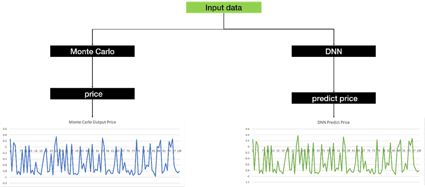
Figure 1. Structure Diagram
Model Introduction
The AI-based approach for the Snowball model employs a DNN (Deep Neural Network) model. It primarily utilizes matmul operations and multiple fully connected layers. By taking various input parameters, it predicts the corresponding option pricing, functioning as a predictive model.
Optical computing chips can accelerate matrix multiplication, thereby boosting the overall DNN inference performance and improving option pricing efficiency.
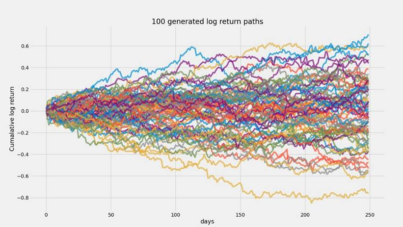
Figure 2. Generation of One Million Paths
[Data Generation]: By running Monte Carlo simulations of the Snowball model with millions of paths under different pricing parameters, the corresponding output prices are obtained to create a dataset. This dataset is then used as training data for the neural network model to predict option pricing.
[Model Construction]: A multi-layer fully connected neural network can be used. The activation functions and the number of neurons in each layer are selected according to the actual situation.
[Model Training]: The training strategy is crucial; a good training strategy yields a model with better fitting. Here, a low-precision quantized model can be adopted, which is more suitable for inference on an optical computing card.
[Testing]: The trained model is tested, and all evaluation metrics must meet practical requirements while ensuring the model’s sensitivity.
Summary
It should be noted that the above steps only outline the use of a DNN-type neural network model for predicting option pricing. This application scenario demands high computational power and computing speed. Therefore, we propose leveraging the low latency and high bandwidth of optical computing to solve the entire problem. Optical computing algorithms can also be hybrid-integrated with classical algorithms to further accelerate problem solving.
References
[1] https://developer.nvidia.com/blog/accelerating-python-for-exotic-option-pricing/
[2] Ferguson R, Green A. Deeply learning derivatives[J]. arXiv preprint arXiv:1809.02233, 2018.


