














Optical computing applied to ResNet50 image classification
1. Dataset Introduction
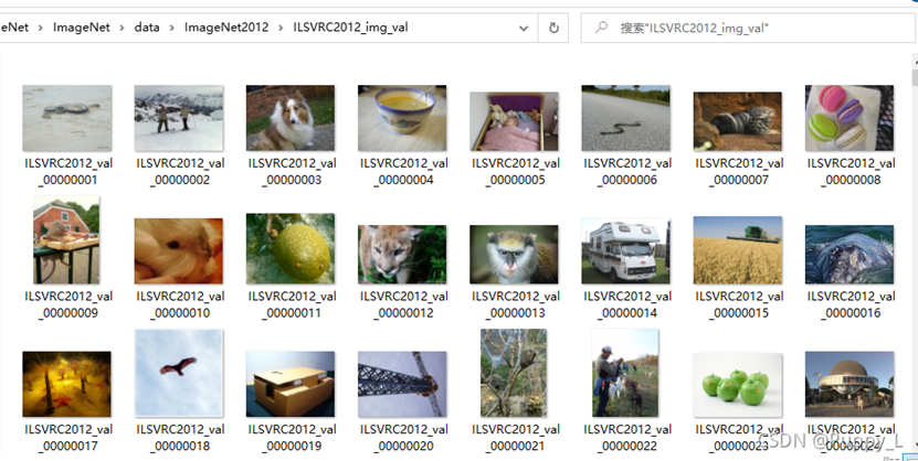
ImageNet is a dataset, not a neural network model. It was created under the leadership of Stanford University Professor Fei-Fei Li to address the overgeneralization and over-generalization problems in machine learning. The dataset was initially developed in 2007 and was officially released as a paper at CVPR 2009. To this day, it remains one of the most commonly used datasets in the field of deep learning for image processing, classification, and localization.
There was a competition based on ImageNet, held annually from 2010 to 2017. This competition, known as ILSVRC (ImageNet Large-Scale Visual Recognition Challenge), used a subset of samples from the ImageNet dataset each year. ILSVRC included challenges in image classification, object localization, object detection, video object detection, and scene classification. Among the past winners were well-known deep learning network models such as AlexNet (2012), VGG (2014), GoogLeNet (2014), and ResNet (2015). The term "ILSVRC" sometimes specifically refers to the dataset used in the competition, a subset of ImageNet, most commonly the 2012 dataset, denoted as ILSVRC2012. Therefore, when referring to ImageNet, it likely means the subset of ImageNet used for ILSVRC2012. The ILSVRC2012 dataset has 1000 categories (meaning the output of a neural network for ImageNet image recognition is 1000), with approximately 1000 images per category. The total number of images used for training is approximately 1.2 million, in addition to some images used as validation and test sets. ILSVRC2012 contains 50,000 images as the validation set and 100,000 images as the test set (the test set is unlabeled; the labels for the validation set are given in a separate document).
2. Network Structure
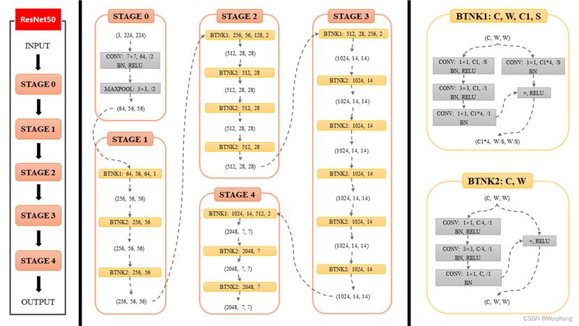
As shown in the figure, the ResNet50 network operates from input -> stage0 -> stage1 -> stage2 -> stage3 -> stage4 -> output.
Stage0 is relatively simple. The input (3, 224, 224) passes through 64 convolutional kernels of size (7, 7) with a stride of 2. At this point, the output channel count is 64 (the number of feature maps output by the convolutional layer equals the number of convolutional kernels). Next, it passes through a Batch Normalization (BN) layer. BN is a regularization technique commonly used in deep neural networks. BN can accelerate the training process of the neural network and make the gradients in the network more stable during backpropagation. ReLU is the activation function. Finally, it passes through a max pooling layer, where the kernel size is 3×3 and the stride is 2. The final output size is 224/2/2 = 56.
Overall, after stage0, the shape changes from (3, 224, 224) -> (64, 56, 56).
3.Model Training
3.1 Data Preprocessing During training, the input data needs to be preprocessed. The code is as follows:
input_size = 224
traindir = os.path.join(args.data, 'train')
valdir = os.path.join(args.data, 'val')
normalize = transforms.Normalize(mean=[0.485, 0.456, 0.406],
std=[0.229, 0.224, 0.225])
# torchvision.set_image_backend('accimage')
train_dataset = datasets.ImageFolder(
traindir,
transforms.Compose([
transforms.Resize(256),
transforms.RandomCrop(input_size),
transforms.RandomHorizontalFlip(),
# AutoAugment(policy=AutoAugmentPolicy.IMAGENET),
transforms.ToTensor(),
normalize,
]))
train_loader = torch.utils.data.DataLoader(
train_dataset, batch_size=args.batch_size, shuffle=True,
num_workers=args.workers, pin_memory=True)
val_loader = torch.utils.data.DataLoader(
datasets.ImageFolder(valdir, transforms.Compose([
transforms.Resize(256),
transforms.CenterCrop(input_size),
transforms.ToTensor(),
normalize,
])),
batch_size=args.batch_size, shuffle=False,
num_workers=args.workers, pin_memory=True)
The args.data parameter is the path to the dataset. Input should be set to size 224.。
3.2 Loss Function and Optimizer
The code is as follows:
criterion = nn.CrossEntropyLoss().cuda(args.gpu)
optimizer = torch.optim.SGD(model.parameters(), lr=args.lr, momentum=0.9, weight_decay=args.weight_decay)
scheduler = torch.optim.lr_scheduler.MultiStepLR(optimizer, milestones=[10, 20, 30, 90, 120], gamma=0.1)
Initialize the learning rate lr = 0.01 and use the cross-entropy loss function.
3.2 QAT Training of Low-Bit Models
3.2.1 Quantization Tool MOCA (Method 1)
This is a quantization tool developed based on mqbench, suitable for quantization in optical computing and conversion of ONNX deployment models. The operators in the ONNX model are custom-defined operators executable by optical computing hardware, suitable for 8/4/3/2-bit fixed-point quantization.
Here, you need to download and install the MOCA tool:
python setup.py develop
and modify the code:
moca/QuantForCV/mqbench/mqbench/prepare_by_platform.py

This is where you configure the quantization type and bit depth.
moca/QuantForCV/mqbench/application/imagenet_example/main.py
This is where main.py is configured, specifying which layers should be executed in OMAC. `omac_exec_layers` is a dictionary that can be configured for either 4-bit or 2-bit quantization. During training, it's important to note that the pre-trained model should be loaded first.
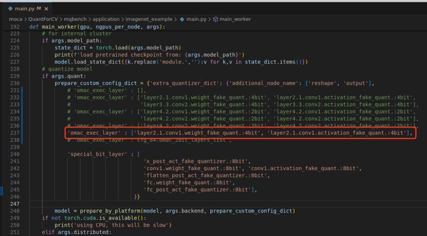
Execute the following command to perform QAT training. Hardware-aware quantization can also be introduced.
CUDA_VISIBLE_DEVICES=0 python -u main.py -a resnet50 --train_data /root/imagenet/
--val_data /root/imagenet/ --epochs 2 --lr 1e-4 -b 16 --backend onnx_omac
--model_path /root/.cache/torch/hub/checkpoints/MEALV2_ResNet50_224_cutmix.pth
> resent50.log 2>&1&
3.2.2 APOT Algorithm Quantization (Method 2)
This paper first proposes Additive Powers-of-Two (APoT) quantization, an efficient non-uniform quantization scheme for bell-shaped and long-tailed neural network weights. By restricting all quantized values to the sum of several powers of two, APoT quantization improves computational efficiency and matches the weight distribution well. Secondly, this paper parameterizes the Clipping function to generate better gradients for updating the optimal saturation threshold. Finally, weight normalization is proposed to adjust the input distribution of the weights, making it more stable and consistent after quantization. Experimental results show that the proposed method outperforms state-of-the-art methods and even competes with full-precision models, thus proving the effectiveness of the proposed APoT quantization. For example, the 3-bit quantization of ResNet-34 on ImageNet only reduced Top-1 accuracy by 0.3% and Top-5 accuracy by 0.2%.
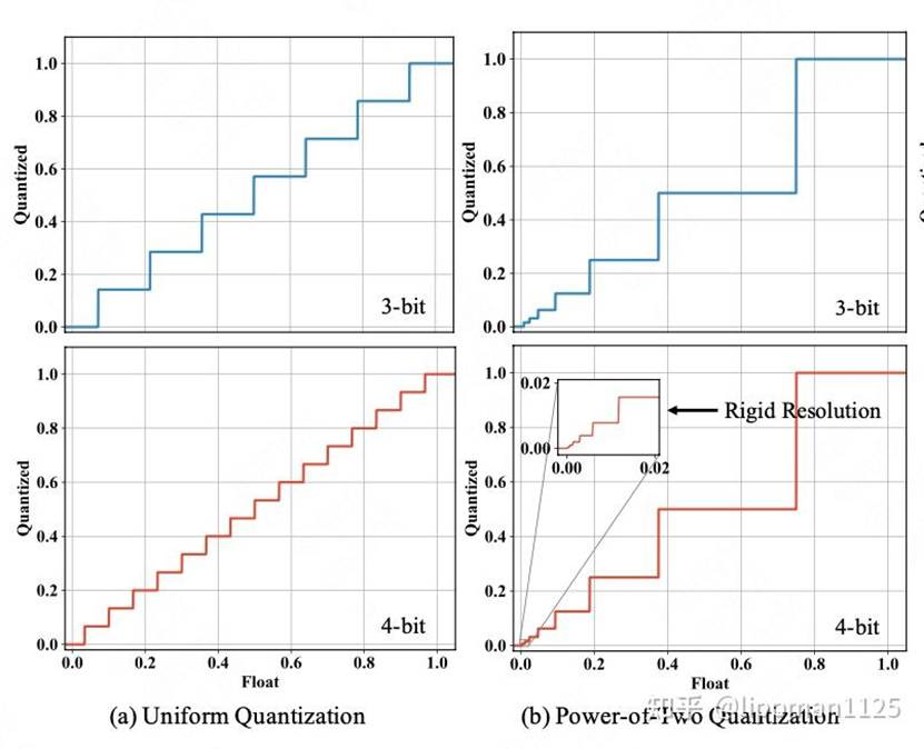
According to the PoT formula, increasing the bitwidth only increases the representation precision near zero, which is wasteful. Therefore, the original text represents the data as the addition of multiple PoTs. The formula is as follows:

For example, quantizing a 4-bit model with b=4, k=2, and n=2 yields two Pots of Time (PoTs), as follows:

Therefore, we obtain 16 discrete values as follows: {0.0000, 0.3333, 0.6667, 0.0833, 0.0208, 1.0000, 0.7500, 0.6875, 0.1667, 0.5000, 0.2500, 0.1875, 0.0417, 0.3750, 0.1250, 0.0625}
Furthermore, we perform a weight normalization operation. Weight normalization provides a relatively consistent and stable input distribution for clipping and projection, which facilitates smoother optimization of different layers and iterations during training. Furthermore, setting the average weight to zero makes quantization more symmetrical. The weight normalization formula is as follows, mainly achieved by subtracting the mean from the weight value and dividing by the variance, so that the normalized weight distribution satisfies a mean of 0 and a variance of 1.

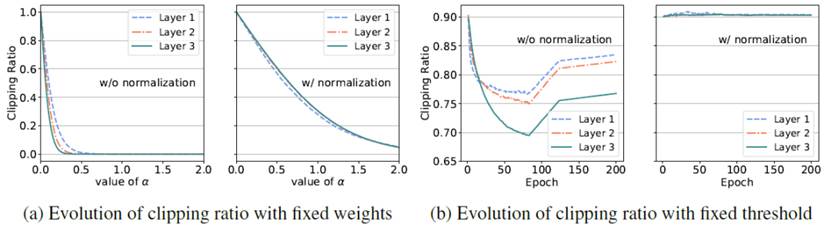
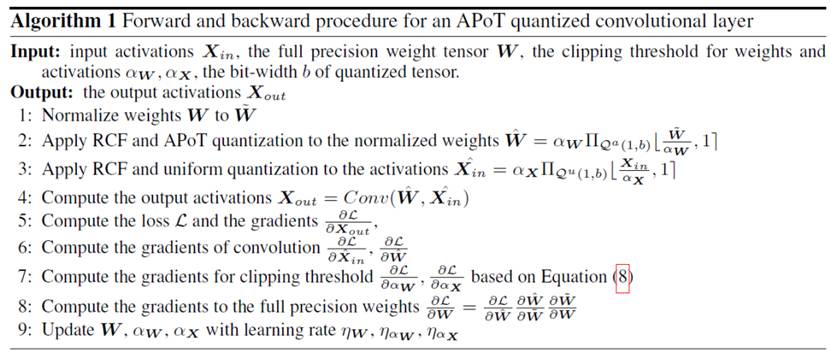
The pseudocode for APoT quantization is as follows:
Project code reference: https://github.com/yhhhli/APoT_Quantization
4. Test Results
w = [-1, 0, 1], a uses uint
w2a2: acc@Top1=72.602% acc@Top5=90.866%
w2a3: acc@Top1=73.434% acc@Top5=91.568%
w3a3: acc@Top1=75.488% acc@Top5=92.532%