Application of optical computing in RetinaNet object detection task

2026.04.02

1. Dataset Introduction

The full name of the DOTA dataset is: Dataset for Object Determination in Aerial Images.

The DOTA dataset v1.0 contains 2806 images of 4000 × 4000 pixels, containing a total of 188282 objects.

DOTA Dataset Paper Introduction: https://arxiv.org/pdf/1711.10398.pdf

Dataset Website:

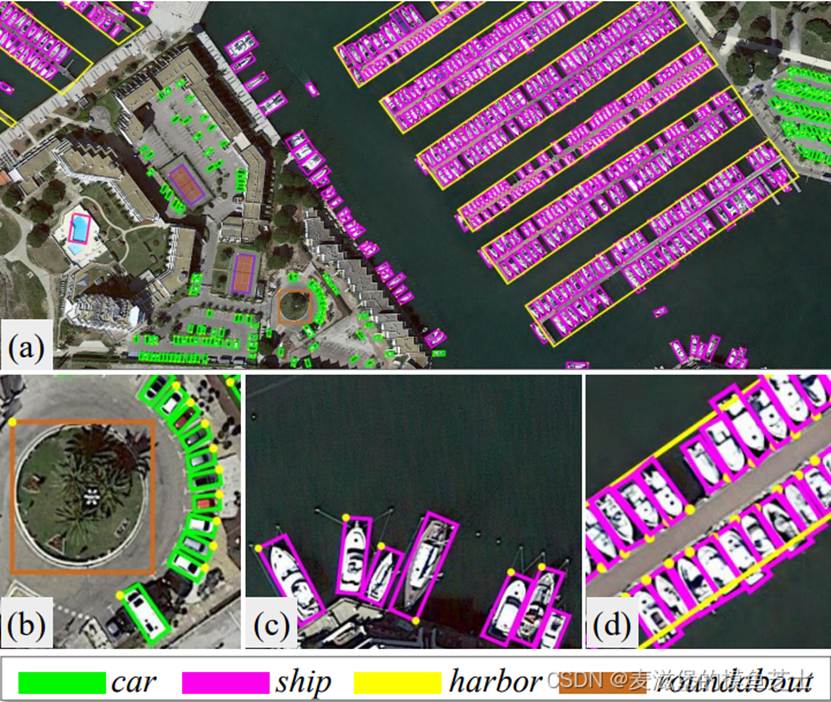
The DOTA dataset has three versions:

* DOTAV1.0

Number of categories: 15

Category names: plane, ship, storage tank, baseball diamond, tennis court, basketball court, ground track field, harbor, bridge, large vehicle, small vehicle, helicopter, roundabout, soccer ball field, swimming pool

* DOTAV1.5

Number of categories: 16

* DOTAV2.0

Number of categories: 18

(1) Labels

When augmenting a dataset, we need to know the relevant label file format.

Each object has 10 values. The first 8 represent the coordinates of the four corners of a rectangle, the 9th represents the object category, and the 10th represents the difficulty level of recognition, with 0 indicating easy and 1 indicating difficult.

Below is a similar file.

950.0 851.0 931.0 852.0 932.0 817.0 952.0 817.0 small-vehicle 1

475.0 982.0 456.0 982.0 461.0 841.0 481.0 842.0 large-vehicle 0

424.0 978.0 400.0 982.0 403.0 840.0 426.0 839.0 large-vehicle 0

395.0 984.0 373.0 985.0 376.0 842.0 399.0 843.0 large-vehicle 0

365.0 979.0 344.0 978.0 346.0 839.0 369.0 838.0 large-vehicle 0

337.0 977.0 317.0 977.0 321.0 836.0 339.0 835.0 large-vehicle 0

310.0 978.0 287.0 979.0 286.0 838.0 311.0 838.0 large-vehicle 0

154.0 947.0 250.0 947.0 250.0 971.0 154.0 971.0 large-vehicle 0

140.0 894.0 255.0 894.0 255.0 919.0 140.0 919.0 large-vehicle 0

116.0 862.0 236.0 862.0 236.0 888.0 116.0 888.0 large-vehicle 0

146.0 771.0 269.0 771.0 269.0 796.0 146.0 796.0 large-vehicle 0

136.0 741.0 271.0 741.0 271.0 766.0 136.0 766.0 large-vehicle 0

136.0 713.0 271.0 713.0 271.0 735.0 136.0 735.0 large-vehicle 0

It can be seen that its label is a rotating box composed of four points. Note: Since the visualization code requires the coordinate point input to be an integer, the coordinate point of the output object is rounded down, which will result in some loss of precision.

(2) Data Augmentation

Related data augmentation, DOTA (obb) data augmentation (methods include: changing brightness, adding noise, rotating angle, mirroring, translating, cropping, cutout), related code is as follows:

2025.8.3: Data Augmentation (dota 4-point conversion)

# -*- coding=utf-8 -*-

# Includes:

# 6. Cropping (requires changing the bbox)

# 5. Translation (requires changing the bbox)

# 1. Changing brightness

# 2. Adding noise

# 3. Rotating angle (requires changing the bbox)

# 4. Mirroring (requires changing the bbox)

# 7. Cutout

# Note:

# random.seed(), the same seed will generate the same random number!!

import time

import random

import cv2 as cv

import os

import math

import numpy as np

from skimage.util import random_noise

from skimage import exposure

import shutil

import imutils

# adujust brightness

def changeLight(img,inputtxt,outputiamge,outputtxt):

# random.seed(int(time.time()))

flag = random.uniform(0.5, 1.5) # flag > 1 means dimming, less than 1 means brightening

label=round(flag,2)

(filepath, tempfilename) = os.path.split(inputtxt)

(filename, extension) = os.path.splitext(tempfilename)

outputiamge=os.path.join(outputiamge+"/"+filename+"_"+str(label)+".jpg")

outputtxt=os.path.join(outputtxt+"/"+filename+"_"+str(label)+extension)

ima_gamma=exposure.adjust_gamma(img, 0.5)

shutil.copyfile(inputtxt, outputtxt)

cv.imwrite(outputiamge,ima_gamma)

# Add noise

def gasuss_noise(image,inputtxt,outputimage,outputtxt,mean=0, var=0.01):

'''

Add Gaussian noise

mean : mean

var : variance

'''

image = np.array(image/255, dtype=float)

noise = np.random.normal(mean, var ** 0.5, image.shape)

out = image + noise

if out.min() < 0:

low_clip = -1.

else:

low_clip = 0.

out = np.clip(out, low_clip, 1.0)

out = np.uint8(out*255)

(filepath, tempfilename) = os.path.split(inputtxt)

(filename, extension) = os.path.splitext(tempfilename)

outputiamge = os.path.join(outputiamge + "/" + filename + "_gasunoise_" + str(mean)+"_"+str(var)+ ".jpg")

outputtxt = os.path.join(outputtxt + "/" + filename + "_gasunoise_" + str(mean)+"_"+str(var)+ extension)

shutil.copyfile(inputtxt, outputtxt)

cv.imwrite(outputiamge, out)

# Contrast Adjustment Algorithm

def ContrastAlgorithm(rgb_img,inputtxt, outputimag, outputtxt):

img_shape=rgb_img.shape

temp_imag=np.zeros(img_shape, dtype=float)

for num in range(0,3):

# Enhance contrast through histogram normalization

in_image =rgb_img[:,:,num]

# Calculate the maximum and minimum pixel values of the input image

Imax = np.max(in_image)

Imin = np.min(in_image)

# The minimum and maximum gray levels to output

Omin, Omax = 0, 255

# Calculate the values of a and b

a = float(Omax - Omin) / (Imax - Imin)

b = Omin - a * Imin

# Linear transformation of the matrix

out_image = a * in_image + b

# Data type conversion

out_image = out_image.astype(np.uint8)

temp_imag[:,:,num]=out_image

(filepath, tempfilename) = os.path.split(inputtxt)

(filename, extension) = os.path.splitext(tempfilename)

outputiamge = os.path.join(outputiamge + "/" + filename + "_contrastAlgorithm" + ".jpg")

outputtxt = os.path.join(outputtxt + "/" + filename + "_contrastAlgorithm" + extension)

shutil.copyfile(inputtxt, outputtxt)

cv.imwrite(outputiamge, temp_imag)

# rotate

def rotate_img_bbox(img, inputtxt,temp_outputiamge,temp_outputtxt,angle,scale=1):

nAgree=angle

size=img.shape

w=size[1]

h=size[0]

for numAngle in range(0,len(nAgree)):

dRot = nAgree[numAngle] * np.pi / 180

dSinRot = math.sin(dRot)

dCosRot = math.cos(dRot)

nw = (abs(np.sin(dRot) * h) + abs(np.cos(dRot) * w)) * scale

nh = (abs(np.cos(dRot) * h) + abs(np.sin(dRot) * w)) * scale

(filepath, tempfilename) = os.path.split(inputtxt)

(filename, extension) = os.path.splitext(tempfilename)

outputiamge = os.path.join(temp_outputiamge + "/" + filename + "_rotate_" + str(nAgree[numAngle])+ ".jpg")

outputtxt = os.path.join(temp_outputtxt + "/" + filename + "_rotate_" + str(nAgree[numAngle])+ extension)

rot_mat = cv.getRotationMatrix2D((nw * 0.5, nh * 0.5), nAgree[numAngle], scale)

rot_move = np.dot(rot_mat, np.array([(nw - w) * 0.5, (nh - h) * 0.5, 0]))

rot_mat[0, 2] += rot_move[0]

rot_mat[1, 2] += rot_move[1]

# Affine transformation

rotat_img = cv.warpAffine(img, rot_mat, (int(math.ceil(nw)), int(math.ceil(nh))), flags=cv.INTER_LANCZOS4)

cv.imwrite(outputiamge,rotat_img)

save_txt=open(outputtxt,'w')

f = open(inputtxt)

for line in f.readlines():

line= line.split(" ")

x1=float(line[0])

y1=float(line[1])

x2 = float(line[2])

y2 = float(line[3])

x3 = float(line[4])

y3 = float(line[5])

x4 = float(line[6])

y4 = float(line[7])

category=str(line[8])

point1 = np.dot(rot_mat, np.array([x1, y1, 1]))

point2 = np.dot(rot_mat, np.array([x2, y2, 1]))

point3 = np.dot(rot_mat, np.array([x3, y3, 1]))

point4 = np.dot(rot_mat, np.array([x4, y4, 1]))

x1=round(point1[0],3)

y1 = round(point1[1], 3)

x2 = round(point2[0], 3)

y2 = round(point2[1], 3)

x3 = round(point3[0], 3)

y3 = round(point3[1], 3)

x4 = round(point4[0], 3)

y4 = round(point4[1], 3)

string = str(x1) + " " + str(y1) + " " + str(x2) + " " + str(y2) + " " + str(x3) + " " + str(

y3) + " " + str(x4) + " " + str(y4)+" "+category

save_txt.write(string)

def filp_pic_bboxes(img, inputtxt,outputiamge,outputtxt):

# ---------------------- Flip image ----------------------

(filepath, tempfilename) = os.path.split(inputtxt)

(filename, extension) = os.path.splitext(tempfilename)

output_vert_flip_img = os.path.join(outputiamge + "/" + filename + "_vert_flip" + ".jpg")

output_vert_flip_txt = os.path.join(outputtxt + "/" + filename + "_vert_flip" + extension)

output_horiz_flip_img = os.path.join(outputiamge + "/" + filename + "_horiz_flip" + ".jpg")

output_horiz_flip_txt = os.path.join(outputtxt + "/" + filename + "_horiz_flip" + extension)

h,w,_ = img.shape

#vertical flip vert_flip_img = cv.flip(img, 1)

cv.imwrite(output_vert_flip_img,vert_flip_img)

# Flip horizontally

horiz_flip_img = cv.flip(img, 0)

cv.imwrite(output_horiz_flip_img,horiz_flip_img)

# ---------------------- Adjust boundingbox ----------------------

save_vert_txt = open(output_vert_flip_txt, 'w')

save_horiz_txt = open(output_horiz_flip_txt, 'w')

f = open(inputtxt)

for line in f.readlines():

line = line.split(" ")

x1 = float(line[0])

y1 = float(line[1])

x2 = float(line[2])

y2 = float(line[3])

x3 = float(line[4])

y3 = float(line[5])

x4 = float(line[6])

y4 = float(line[7])

category = str(line[8])

horiz_string = str(round(w-x1,3)) + " " + str(y1) + " " + str(round(w-x2,3)) + " " + str(y2) + " " + str(round(w-x3,3)) + " " + str(y3) + " " + str(

round(w - x4, 3)) + " " + str(y4) + " " + category

vert_string = str(x1) + " " + str(round(h-y1,3)) + " " + str(x2) + " " + str(round(h-y2,3)) + " " + str(x3) + " " + str(

round(h - y3, 3)) + " " + str(x4) + " " + str(round(h-y4,3)) + " " + category

save_horiz_txt.write(vert_string)

save_vert_txt.write(horiz_string)

#Translate the image

def shift_pic_bboxes(img, inputtxt,outputiamge,outputtxt):

# ---------------------- Translate the image ----------------------

w = img.shape[1]

h = img.shape[0]

x_min = w # The smallest box containing all target boxes after cropping

x_max = 0

y_min = h

y_max = 0

f = open(inputtxt)

for line in f.readlines():

line = line.split(" ")

x1 = float(line[0])

y1 = float(line[1])

x2 = float(line[2])

y2 = float(line[3])

x3 = float(line[4])

y3 = float(line[5])

x4 = float(line[6])

y4 = float(line[7])

category = str(line[8])

x_min = min(x_min, x1,x2,x3,x4)

y_min = min(y_min, y1,y2,y3,y4)

x_max = max(x_max, x1,x2,x3,x4)

y_max = max(y_max, y1,y2,y3,y4)

d_to_left = x_min # Maximum leftward movement distance including all target boxes

d_to_right = w - x_max # Maximum rightward movement distance including all target boxes

d_to_top = y_min # Maximum upward movement distance including all target boxes

d_to_bottom = h - y_max # Maximum downward movement distance including all target boxes

x = random.uniform(-(d_to_left - 1) / 3, (d_to_right - 1) / 3)

y = random.uniform(-(d_to_top - 1) / 3, (d_to_bottom - 1) / 3)

(filepath, tempfilename) = os.path.split(inputtxt)

(filename, extension) = os.path.splitext(tempfilename)

if x>=0 and y>=0 :

outputiamge = os.path.join(outputiamge + "/" + filename + "_shift_" + str(round(x,3))+"_"+str(round(y,3)) + ".jpg")

outputtxt = os.path.join(outputtxt + "/" + filename + "_shift_" + str(round(x,3))+"_"+str(round(y,3)) + extension)

elif x>=0 and y<0:

outputiamge = os.path.join(

outputiamge + "/" + filename + "_shift_" + str(round(x, 3)) + "__" + str(round(abs(y), 3)) + ".jpg")

outputtxt = os.path.join(

outputtxt + "/" + filename + "_shift_" + str(round(x, 3)) + "__" + str(round(abs(y), 3)) + extension)

elif x<0 and="" y="">=0:

outputiamge = os.path.join(

outputiamge + "/" + filename + "_shift__" + str(round(abs(x), 3)) + "_" + str(round(y, 3)) + ".jpg")

outputtxt = os.path.join(

outputtxt + "/" + filename + "_shift__" + str(round(abs(x), 3)) + "_" + str(round(y, 3)) + extension)

elif x<0 and y<0:

outputiamge = os.path.join(

outputiamge + "/" + filename + "_shift__" + str(round(abs(x), 3)) + "__" + str(round(abs(y), 3)) + ".jpg")

outputtxt = os.path.join(

outputtxt + "/" + filename + "_shift__" + str(round(abs(x), 3)) + "__" + str(round(abs(y), 3)) + extension)

save_txt = open(outputtxt, "w")

f = open(inputtxt)

for line in f.readlines():

line = line.split(" ")

x1 = float(line[0])

y1 = float(line[1])

x2 = float(line[2])

y2 = float(line[3])

x3 = float(line[4])

y3 = float(line[5])

x4 = float(line[6])

y4 = float(line[7])

category = str(line[8])

crop_str = str(round(x1-crop_x_min, 3)) + " " + str(round(y1-crop_y_min, 3)) + " " + str(round(x2-crop_x_min, 3)) + " " + str(\

round(y2-crop_y_min, 3)) + " " + str(round(x3-crop_x_min, 3)) + " " + str(round(y3-crop_y_min, 3)) + " " + str(\

round(x4-crop_x_min, 3)) + " " + str(round(y4-crop_y_min, 3)) + " " + category

save_txt.write(crop_str)

if __name__=='__main__':

inputiamge="./split_data_overlap512/agumnet_data/images"

inputtxt = "./split_data_overlap512/agumnet_data/labels"

outputiamge = "./split_data_overlap512/agumnet_data/images"

outputtxt = "./split_data_overlap512/agumnet_data/labels"

angle=[30,60,90,120,150,180]

tempfilename=os.listdir(inputiamge)

for file in tempfilename:

(filename,extension)=os.path.splitext(file)

input_image=os.path.join(inputiamge+"/"+file)

input_txt=os.path.join(inputtxt+"/"+filename+".txt")

img = cv.imread(input_image)

# Image brightness change

# changeLight(img, input_txt, outputiamge, outputtxt)

# Add Gaussian noise

# gasuss_noise(img, input_txt, outputiamge, outputtxt, mean=0, var=0.001)

# Change image contrast

# ContrastAlgorithm(img, input_txt, outputiamge, outputtxt)

# Image rotation

# rotate_img_bbox(img, input_txt, outputiamge, outputtxt, angle)

# Image mirroring

filp_pic_bboxes(img, input_txt, outputiamge, outputtxt)

# Translation

# shift_pic_bboxes(img, input_txt, outputiamge, outputtxt)

# Cropping

# crop_img_bboxes(img, input_txt, outputiamge, outputtxt)

print("###finished!!!")

```

2. Model

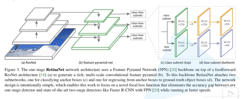
The original RetinaNet paper, published at ICCV 2017, is titled "Focal Loss for Dense Object Detection." It was the first one-stage network to surpass a two-stage network, winning the best student paper award, despite not making any groundbreaking contributions to the network structure.

2.1 backbone

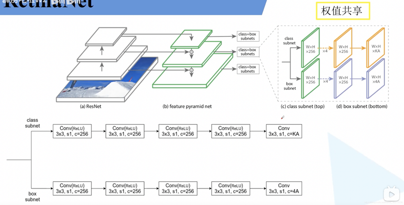
The detailed structure of the RetinaNet network is shown below. Unlike FPN, which uses C2, RetinaNet does not, because P2 generated by C2 would consume more computational resources. Therefore, the authors directly started generating P3 from C3. The backbone part is basically similar to that of FPN, so the specific details will not be discussed further. The second difference lies in P6. The original paper generated it based on C5 (obtained by max pooling downsampling). Here, it is drawn according to the official PyTorch implementation, which uses 3 x 3 convolutional layers to achieve downsampling. The third difference is that FPN goes from P2 to P6, while RetinaNet goes from P3 to P7.

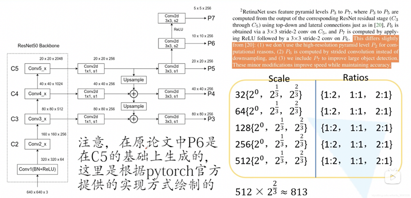
The figure above also shows the scales and ratios used from P3 to P7. In FPN, one scale and three ratios are used on each feature layer. In RetinaNet, there are three scales and three ratios, totaling 9 anchors. Note that here, the area of the anchor corresponding to a scale of 32 is the square of 32. Therefore, the smallest scale in RetinaNet is 32, and the largest is close to 813.

2.2 Predictor Section

Since RetinaNet is a one-stage network, ROI pooling is not used; instead, a weight-sharing convolution-based predictor is used directly, as shown in the figure below. The predictor is divided into two branches: predicting the class of each anchor and the regression parameters of the target bounding box. In the final kA, k is the number of target classes detected; note that k here does not include the background class, which is 20 for the PASCAL VOC dataset. A here is the number of anchors generated at each position of the predicted feature layer, which is 9 in this case. (Currently, most anchor regression parameter predictions are of this kind, which can also be understood as each class sharing the same anchor regression parameter predictor.)

2.3 Positive and Negative Sample Matching

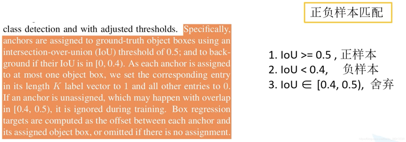
For each anchor, it is compared with the pre-labeled ground truth boxes. If the IoU is greater than 0.5, it is a positive sample. If the IoU of an anchor with all ground truth boxes is less than 0.4, it is a negative sample. The rest are discarded.

2.4 Loss Calculation

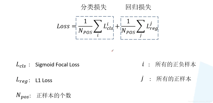
A core contribution of this paper is the focal loss. The total loss is still divided into two parts: classification loss and regression loss. A unique aspect of focal loss is that the classification loss is calculated for both positive and negative samples, while the regression loss is calculated only for positive samples. Regression loss is explained in SSD and Faster R-CNN.

2.5 Focal Loss

To achieve a balanced ratio of positive to negative samples and prevent the entire training process from being "overwhelmed" by negative samples, a sampling method is generally used to control the ratio of positive to negative samples at 1:3, thus maintaining a reasonable proportion between positive and negative samples. Because one-stage training only has one phase, it generates far more candidate boxes than two-stage training. Typically, it requires approximately 100K locations (e.g., 8700+ locations in SSD), and among these, only a few (a dozen or so) are positive samples. Even with sampling, during the training process, you will still be surprised to find that the entire process is still dominated by a large number of easily distinguishable negative samples, i.e., the background. Focal loss is a dynamically scaled cross-entropy loss. In short, through a dynamic scaling factor, it can dynamically reduce the weight of easily distinguishable samples during training, thereby quickly focusing the loss on those difficult-to-distinguish samples (note: difficult-to-distinguish samples are not necessarily positive samples).

2.6 Cross Entropy Loss

The origin of Focal loss is binary cross-entropy (CE), which takes the following form:：

In the above formula, y can take the values 1 and -1, representing foreground and background, respectively. p ranges from [0,1] and represents the probability of belonging to the foreground predicted by the model. For convenience, a value pt is defined.

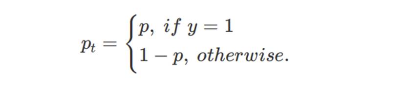
Combining equations (1) and (2), we can obtain:

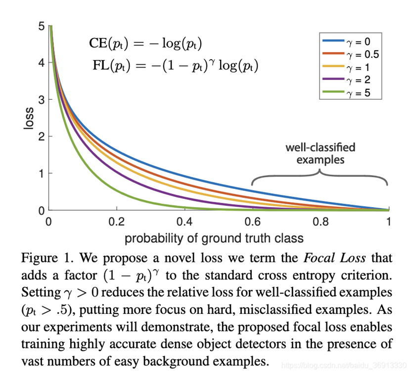
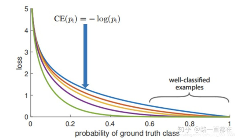
The CE curve is the blue curve in the figure below. As you can see, compared to other curves, the blue line changes the most smoothly. Even when p > 0.5 (which is already a well-distinguished sample), its loss is still high compared to other curves. Although it has decreased a lot compared to the previous ones, when the losses of a huge number of easily distinguishable samples are added together, it will dominate our training process. Therefore, we need to further increase the ratio of the magnitude of the losses before and after.

2.7 Balanced Cross Entropy

Balanced Cross Entropy is a common method for addressing class imbalance. Its idea is to introduce a weight factor α ∈ [0,1]. When the class label is 1, the weight factor is α; when the class label is -1, the weight factor is 1-α. For convenience, we use αt to represent the weight factor. The loss function is then rewritten as:

2.8 Calculation of Focal Loss

Balanced Cross Entropy addresses the imbalance between positive and negative examples, but it only balances the positive and negative samples without distinguishing between easy and hard examples. When easily distinguishable negative examples are abundant, the entire training process revolves around these examples (small losses accumulate and exceed large losses), while the hard-to-distinguish examples are neglected and become the focus of training. The authors introduce a new modulation factor, as shown in the following formula:

γ is also a parameter, ranging from [0,5]. Observing the above formula, we can see that when pt approaches 1, it indicates that the sample is relatively easy to distinguish, and the entire modulation factor (1-pt)^γ approaches 0, meaning the contribution of the loss is very small. If a sample is misclassified, pt is very small, then the modulation factor (1-pt)^γ approaches 1, which has no significant impact on the loss (relative to the basic cross-entropy). The parameter γ can adjust the rate of weight decay. As shown in the figure below, when γ = 0, $FL$ is the original cross-entropy loss CE. As γ increases, the adjustment rate also changes. Experiments show that the effect is best when γ = 2.

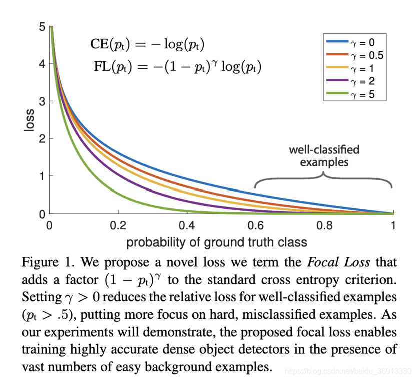
Combining positive/negative sample balance and easy/difficult sample balance, the final Focal loss form is as follows:

Its function can be interpreted as: αt suppresses the imbalance in the number of positive/negative samples, and γ controls the imbalance in the number of easy/difficult samples.

For Focal loss, the following can be summarized:

* For both foreground and background classes, the larger pt is, the smaller the weight (1-pt)^γ, meaning the loss of easy samples can be suppressed by the weights;

* αt is used to adjust the ratio between the losses of positive and negative samples. When αt is used for the foreground class, 1-αt is used for the corresponding background class;

* The optimal values of γ and αt are interdependent, so they need to be adjusted together when evaluating accuracy. The authors in the paper give that RetinaNet with ResNet-101+FPN as the backbone has the best performance when γ=2 and αt=0.25. Here, αt=0.25, with a small weight for positive samples and a large weight for negative samples, is beneficial for reducing the classification loss of negative samples, minimizing the loss of negative samples as much as possible.

3. Model Quantization

Model quantization is the process of converting a floating-point model to a fixed-point model using a certain method. For example, if the original model uses float32 weights, model quantization transforms it into a fixed-point model where all weights are ints.

3.1 Quantization Tool MOCA

This is a quantization tool developed based on mqbench, suitable for quantization in optical computing and for converting deployed ONNX models. The operators in the ONNX model are custom-defined operators executable by optical computing hardware, suitable for 8/4/3/2-bit fixed-point quantization.

3.2 Environment Dependencies

2. Environment Installation

1. This mainly involves installing the mmrotate repository and moca_cv (mqbench and omac). The specific package versions are as follows:

Package Version Editable project location

-------------------------------- ------------ ------------------------------

accimage 0.2.0

addict 2.4.0

aliyun-python-sdk-core 2.15.2

aliyun-python-sdk-kms 2.16.5

appdirs 1.4.4

backports-datetime-fromisoformat 2.0.0

backports.weakref 1.0.post1

certifi 2024.7.4

cffi 1.17.1

charset-normalizer 3.3.2

click 8.1.7

cmake 3.21.0

colorama 0.4.6

coloredlogs 15.0.1

coverage 7.4.3

crcmod 1.7

cryptography 43.0.1

cycler 0.12.1

Cython 3.0.0

e2cnn 0.2.3

easydict 1.9

et-xmlfile 1.1.0

exceptiongroup 1.2.1

filelock 3.14.0

flatbuffers 24.3.25

graphviz 0.20.3

humanfriendly 10.0

idna 3.7

imageio 2.9.0

importlib_metadata 8.5.0

iniconfig 2.0.0

Jinja2 3.1.4

jmespath 0.10.0

joblib 1.2.0

jsonpickle 3.0.1

kiwisolver 1.4.5

lgt_license 1.2.3

lightning-utilities 0.11.7

llvmlite 0.31.0

lvis 0.5.3

Mako 1.3.2

Markdown 3.7

markdown-it-py 3.0.0

MarkupSafe 2.1.3

matplotlib 3.3.3

mdurl 0.1.2

mkl-fft 1.3.8

mkl-random 1.2.4

mkl-service 2.4.0

mmcv 2.0.0rc4

mmcv-full 1.7.2

mmdet 2.28.2 /local/miniconda/envs/moca_cv/lib/python3.8/site-packages

mmengine 0.10.4

mmrotate 0.3.4 /root/dota_workspace/mmrotate

model-index 0.1.11

mpmath 1.3.0

MQBench 0.0.6 /root/workspace_moca_shankun_new/moca/QuantForCV/mqbench

networkx 3.1

ninja 1.11.1.1

numba 0.48.0

numpy 1.22.4

onnx 1.16.0

onnxruntime 1.19.2

onnxsim 0.4.36

opencv-python 4.1.2.30

opendatalab 0.0.10

openmim 0.3.9

openpyxl 3.0.9

openxlab 0.1.1

ordered-set 4.1.0

osimulator 1.2.3

oss2 2.17.0

packaging 24.0

pandas 0.25.3

Pillow 6.2.1

pip 23.3.1

platformdirs 3.10.0

pluggy 1.5.0

prettytable 3.10.0

protobuf 3.20.3

psutil 5.9.0

pycocotools 2.0.7

pycparser 2.22

pycryptodome 3.18.0

pycuda 2024.1

Pygments 2.18.0

pyparsing 3.1.2

pytest 7.4.3

pytest-cov 4.1.0

pytest-html 4.0.2

pytest-metadata 3.1.1

pytest-runner 6.0.1

python-dateutil 2.9.0.post0

pytools 2024.1.6

pytz 2023.4

PyWavelets 1.4.1

PyYAML 6.0.1

requests 2.28.2

rich 13.4.2

scikit-image 0.19.3

scikit-learn 1.3.2

scipy 1.6.3

setuptools 60.2.0

shapely 2.0.6

SharedArray 3.2.1

six 1.16.0

sympy 1.13.2

tabulate 0.9.0

tensorboardX 1.8

termcolor 2.4.0

terminaltables 3.1.10

threadpoolctl 3.5.0

tifffile 2023.7.10

tomli 2.0.1

torch 1.10.1+cu113

torchaudio 0.10.1+cu113

torchmetrics 1.4.1

torchvision 0.11.2+cu113

tqdm 4.65.2

typing_extensions 4.11.0

urllib3 1.26.20

wcwidth 0.2.13

wheel 0.43.0

yapf 0.40.2

zipp 3.20.2

Note: Here, `mqbench` refers to the toolkit for installing MOCA.

3.3 Executing the Program

QAT quantization execution program, low-bit training and quantization

First, QAT needs to be configured in the `train.py` file located at `/root/dota_workspace/mmrotate/mmrotate/apis/train.py`.

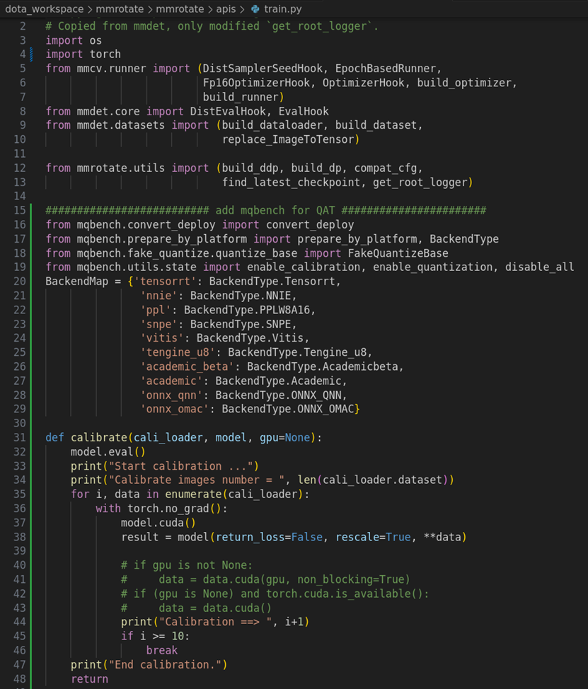
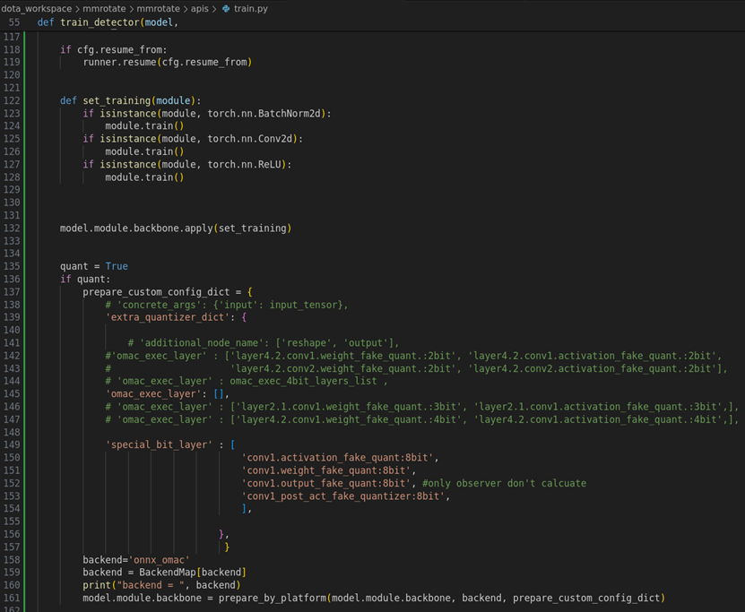
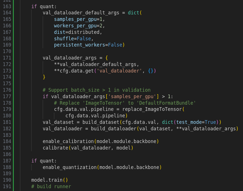
QAT training script for 4-bit models:

CUDA_VISIBLE_DEVICES=0 python -u tools/train.py configs/

rotated_retinanet/rotated_retinanet_obb_r50_fpn_1x_dota_ms_rr_le90.py

--resume-from checkpoints

rotated_retinanet_obb_r50_fpn_1x_dota_ms_rr_le90-1da1ec9c.pth --work-dir logs/train_epoch_35/

> train_log_epoch35.log 2>&1 &

Configuration file:

rotated_retinanet_obb_r50_fpn_1x_dota_ms_rr_le90.py

Pre-trained model:

rotated_retinanet_obb_r50_fpn_1x_dota_ms_rr_le90-1da1ec9c.pth

Training log saving:

logs/train_epoch_35/

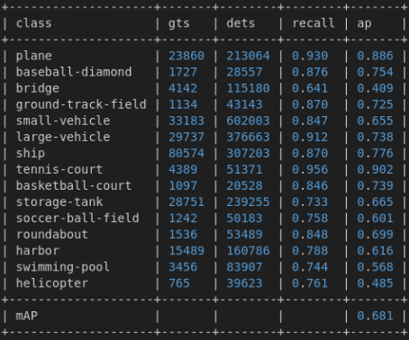
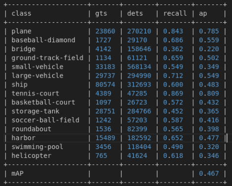
3.4 Training results

(1) For a 1024x1024 input:

(2)For 512x512 input:

4. Test Results on the Optical Computing Simulator

Inference Script Execution:

CUDA_VISIBLE_DEVICES=3 python -u tools/test_qat.py

configs/rotated_retinanet/ rotated_retinanet_obb_r50_fpn_1x_dota_ms_rr_le90.py

checkpoints/epoch_15.pth --eval mAP > test_alllayers.log 2>&1 &

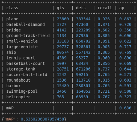
4.1 For a 1024x1024 input, the Compass simulator was used.

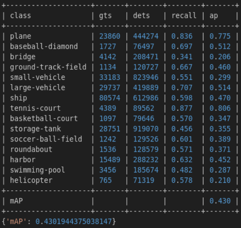
4.2 For a 512x512 input，the Compass simulator was used.

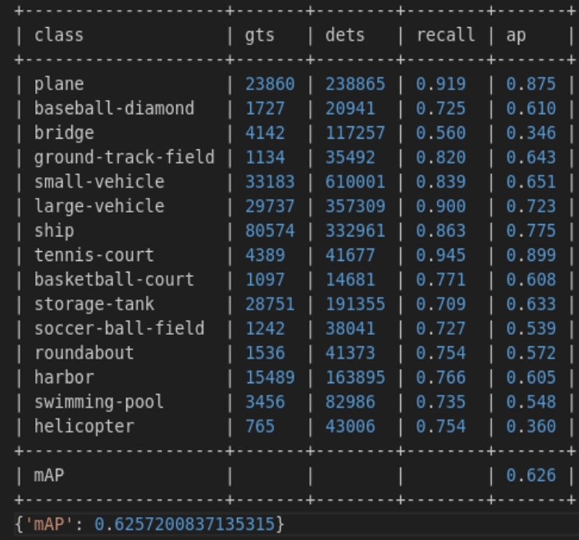
4.3 For a 1024x1024 input ，the Compass simulator was used.

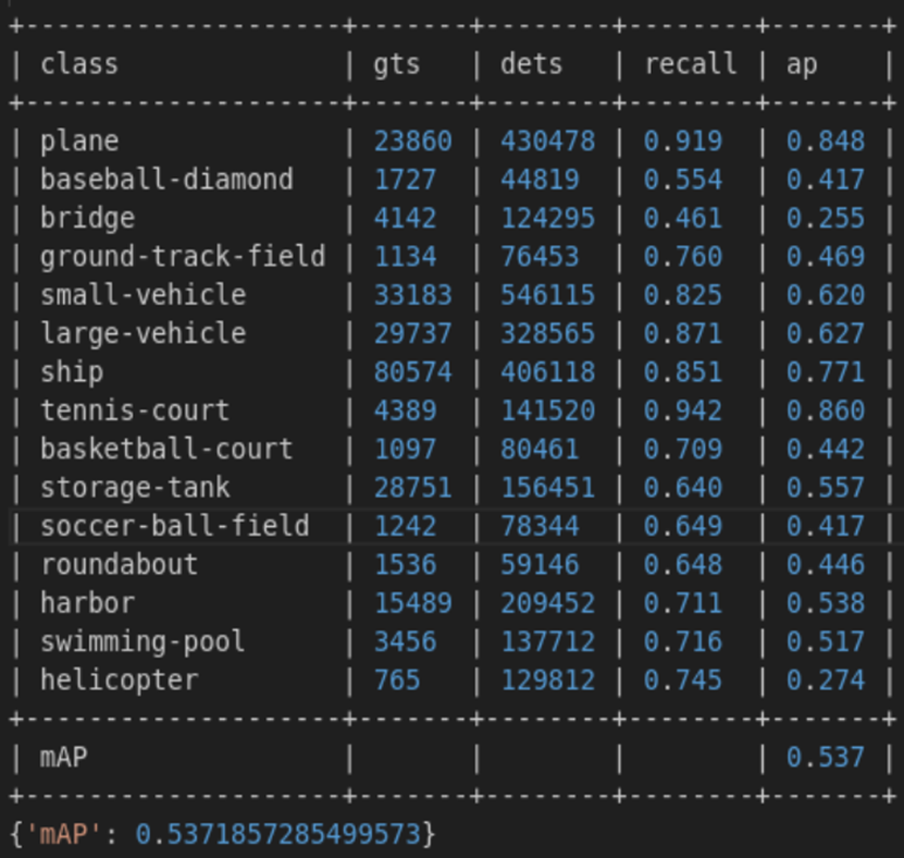
4.4 For a 512x512 input ，the Compass simulator was used.

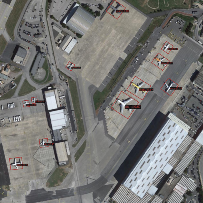
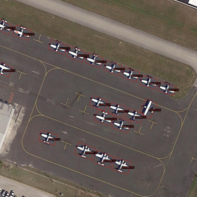
4.5 Test visualization on the optical computing simulator

Back to list